Cooley, Tukey, and the Fast Fourier Transform
Abstract
The Fast Fourier Transform computes the frequency content of a signal of N samples in about N·log N operations instead of N². Its modern form came out of Cold War arms control: at a 1963 meeting of President Kennedy’s Science Advisory Committee on detecting Soviet underground nuclear tests, the Princeton statistician John Tukey sketched the method, the IBM physicist Richard Garwin saw what it was worth, and IBM’s James Cooley programmed it. Their paper of April 1965 turned computations that had taken hours into ones that took seconds, and IBM placed the method in the public domain. The FFT became the core of digital signal processing, from seismology and radar to MP3 audio, medical scanners, Wi-Fi and mobile networks, and in 2000 it was named one of the ten algorithms of the century. Only afterwards did historians find that Carl Friedrich Gauss had used essentially the same method around 1805, in a Latin manuscript published after his death.
Hearing the Frequencies
The Fourier transform decomposes a signal into the frequencies it contains. It is the mathematical operation behind spectrum analyzers, audio and image compression, radar, sonar and radio receivers. For a sampled signal of N values, the discrete Fourier transform (DFT) computes N frequency components, each a weighted sum of all N samples, so a direct computation takes on the order of N² multiplications. For a thousand samples that is a million multiplications; for a million samples, a trillion. In the early 1960s the long records produced by networks of seismometers, radar systems and laboratory instruments made frequency analysis the right tool in principle and unaffordable in practice.
The idea of the fast method is divide and conquer. If N is even, the DFT of N samples can be computed from the DFTs of the even-numbered and the odd-numbered samples, each of length N/2, plus N/2 extra multiplications to combine them. Repeating the split until the pieces have length one gives a total of about N·log₂N operations. For a million samples that is about 20 million instead of a trillion.
DFT cost, N = 1,000,000 samples:

  Direct:        N² = 10¹²  operations
  Cooley–Tukey:  N·log₂N ≈ 2×10⁷ operations

  Speed-up: about 50,000 times
Arms Control
In August 1963 the United States, Britain and the Soviet Union signed the Partial Test Ban Treaty, which banned nuclear tests in the atmosphere, in space and under water but not underground, largely because no one could yet reliably tell an underground explosion from an earthquake at a distance. A comprehensive ban would require a worldwide network of seismometers and the computing power to analyze their records.
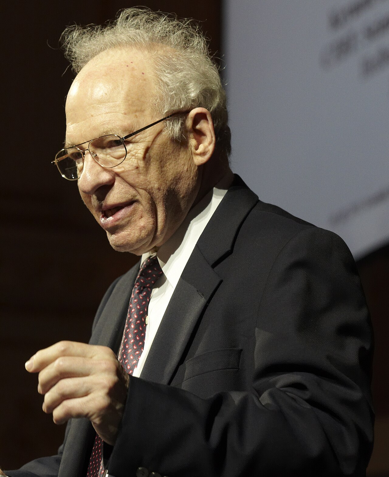
That year John W. Tukey, a Princeton statistician who also worked at Bell Labs and had coined the word “bit”, sat on a panel of President Kennedy’s Science Advisory Committee discussing exactly this problem. During the meetings he worked out a way to compute the DFT recursively in N·log N operations. Richard Garwin, an IBM physicist who had produced the working design of the first hydrogen bomb and was now an adviser on arms control, was at the same meetings. He saw that the method mattered far beyond seismology, and he asked IBM’s research division for someone to program it.
Cooley at IBM
The job went to James W. Cooley, a mathematician at IBM’s Thomas J. Watson Research Center. Because the seismic application was classified, Garwin did not explain it; Cooley later recalled that Garwin told him he wanted the program to determine the periodicities of spin orientations in a three-dimensional crystal of helium-3. Cooley worked out the details of a general algorithm with Tukey, programmed it in 1964 on an IBM 7094, and demonstrated a speed-up of about a hundred times over the direct method on the problem sizes of the day.
Their paper, “An Algorithm for the Machine Calculation of Complex Fourier Series”, appeared in Mathematics of Computation in April 1965. Garwin pushed for wide distribution, and IBM decided to place the algorithm in the public domain rather than patent it. Cooley spent much of the following years explaining it at conferences, including the Arden House workshops on FFT processing in New York, organized by the IEEE Audio and Electroacoustics group in 1968 and 1970, which helped spread it among engineers. The paper became one of the most cited in applied mathematics.
Asked by IEEE Spectrum in 2024 which of his IBM contributions he was proudest of, Garwin named the FFT: “I was the midwife for that. I didn’t invent it. I just sat next to John Tukey.” The IEEE made the first demonstration of the FFT a Milestone, and plaques were dedicated at Princeton on 22 May 2025 and at IBM’s Yorktown Heights laboratory on 11 June 2025.
Gauss Got There First
The 160-year anticipation
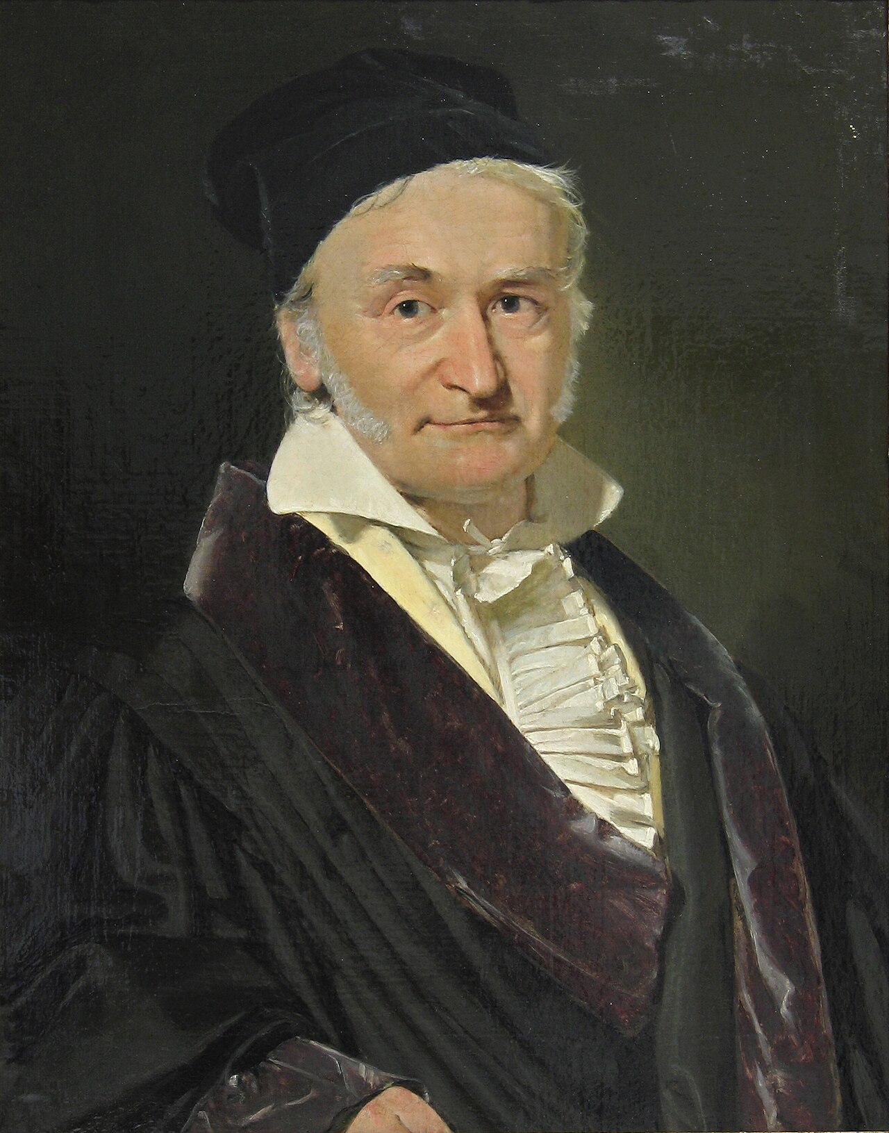
After the 1965 paper’s success, researchers looked for earlier versions and found several. Gordon Danielson and Cornelius Lanczos had published a doubling method in 1942, and others had used related tricks for hand calculation. In 1984 Michael Heideman, Don Johnson and Sidney Burrus showed in “Gauss and the History of the Fast Fourier Transform” that Carl Friedrich Gauss had used essentially the same divide-and-conquer method around 1805, to interpolate the orbits of the asteroids Pallas and Juno from observations, before Joseph Fourier had presented his own work on the series named after him. Gauss wrote it in a Latin treatise that he did not publish; it appeared only in his collected works after his death, where nobody connected it with computing. Before electronic computers, the method saved hours of hand calculation; afterwards it saved orders of magnitude.
What the FFT Made Possible
Within a few years of 1965 the FFT turned the Fourier transform from a theoretical tool into a routine computation, and digital signal processing became a field of its own. Seismologists used it for the test-ban monitoring that had motivated it. Laboratories built FFT-based spectrum analyzers. Radar and sonar systems processed returns in real time. Computed tomography and magnetic resonance imaging reconstruct their images with Fourier methods. Fast convolution by FFT made large digital filters practical. Audio and image compression rests on close relatives: MP3 uses a modified discrete cosine transform and JPEG an 8-by-8 discrete cosine transform, both computed with FFT-like algorithms (see Data Compression). Modern wireless and wired communication, from Wi-Fi and 4G and 5G mobile networks to DSL and digital television, uses orthogonal frequency-division multiplexing (OFDM), in which every transmitter and receiver performs an FFT on every symbol.
In January 2000 the journal Computing in Science & Engineering named the FFT one of the “top ten algorithms of the century”, with the greatest influence on the development and practice of science and engineering (see The Algorithm as a Concept).
Later Algorithms
The original radix-2 algorithm was only the beginning. Researchers developed versions for lengths that are not powers of two, split-radix and prime-factor algorithms, and Winograd’s algorithms that minimize multiplications. As processors grew more complex, the fastest FFT for a given machine became hard to predict. In 1997 Matteo Frigo and Steven G. Johnson at MIT released FFTW (“the Fastest Fourier Transform in the West”), which generates many specialized code fragments and measures which combination runs fastest on the machine at hand. It won the J. H. Wilkinson Prize for Numerical Software in 1999 and became the standard FFT library in scientific software.
James Cooley (1926–2016) spent his career at IBM and became the FFT’s historian. John Tukey (1915–2000) is remembered as much for exploratory data analysis and the box plot as for the FFT. Richard Garwin died on 13 May 2025, aged 97.
Dead End
Gauss’s method is the dead end in this story: a working fast Fourier algorithm, used for real astronomical calculations, that disappeared for a century and a half because it was never published in a form anyone read. Danielson and Lanczos’s 1942 version met a similar fate, appearing in a physics journal when computation was still done by hand and the savings seemed modest. The algorithm became influential only when two conditions met in 1965: computers that could exploit an N/log N advantage, and an author and employer who published it openly and promoted it. The mathematics had been ready since 1805.
📚 Sources
- Cooley, J. W., and Tukey, J. W.: “An Algorithm for the Machine Calculation of Complex Fourier Series”, Mathematics of Computation 19 (April 1965)
- Wikipedia: Cooley–Tukey FFT algorithm
- ETHW: Milestones: First Demonstration of the Fast Fourier Transform (FFT), 1964
- IEEE Spectrum, “FFT: The 60-Year-Old Algorithm Underlying Today’s Tech”: 100-fold speed-up, Milestone dedications 2025
- IBM Research blog, “How IBM Research first demonstrated the revolutionary Cooley-Tukey FFT”: Garwin and Tukey at the 1963 PSAC meeting, Garwin’s introduction
- Cooley, J. W.: “How the FFT Gained Acceptance”, ACM Conference on the History of Scientific and Numeric Computation (1987) and ETHW: Oral history of James W. Cooley: the helium-3 explanation, public domain, Arden House workshops (1968, 1970)
- Heideman, M. T., Johnson, D. H., Burrus, C. S.: “Gauss and the History of the Fast Fourier Transform”, IEEE ASSP Magazine 1(4): 14–21 (1984)
- Daniel Rockmore, “The FFT: an algorithm the whole family can use” (2000)
- Dongarra, J., and Sullivan, F.: “Guest Editors’ Introduction: The Top 10 Algorithms”, Computing in Science & Engineering 2(1) (2000)
- Wikipedia: Fastest Fourier Transform in the West and Frigo, M., and Johnson, S. G.: “The Design and Implementation of FFTW3” (2005)
- ETHW: James W. Cooley
- IEEE Spectrum, “Richard Garwin and Building the First Hydrogen Bomb” (September 2024): the “midwife” quote
- Wikipedia: Richard Garwin and Washington Post, “Richard Garwin, science adviser to presidents, dies at 97” (14 May 2025)
- Image: Richard Garwin 2011.jpg by The Official CTBTO Photostream (CC BY 2.0), via Wikimedia Commons