Rudolf Kálmán and the Kalman Filter
Abstract
In 1960 the Hungarian-born mathematician Rudolf E. Kálmán published a recursive method for estimating the true state of a system from noisy measurements. Facing skepticism among electrical engineers, he presented it through the American Society of Mechanical Engineers, and a follow-up paper with Richard Bucy was at first rejected. In the autumn of 1960 Kálmán visited Stanley Schmidt’s group at NASA’s Ames Research Center, which was looking for a way to navigate a spacecraft to the Moon with a small onboard computer. Schmidt’s engineers turned the linear theory into the extended Kalman filter, which ran in simulation by early 1961 and was carried into the Apollo guidance system by MIT’s Instrumentation Laboratory. The filter later went into aircraft and submarine navigation, cruise missiles, GPS receivers, spacecraft docking, weather forecasting and the sensor fusion of every smartphone. Kálmán also introduced the concepts of controllability and observability, which became the foundation of modern control theory. He died in 2016.
Budapest to Baltimore
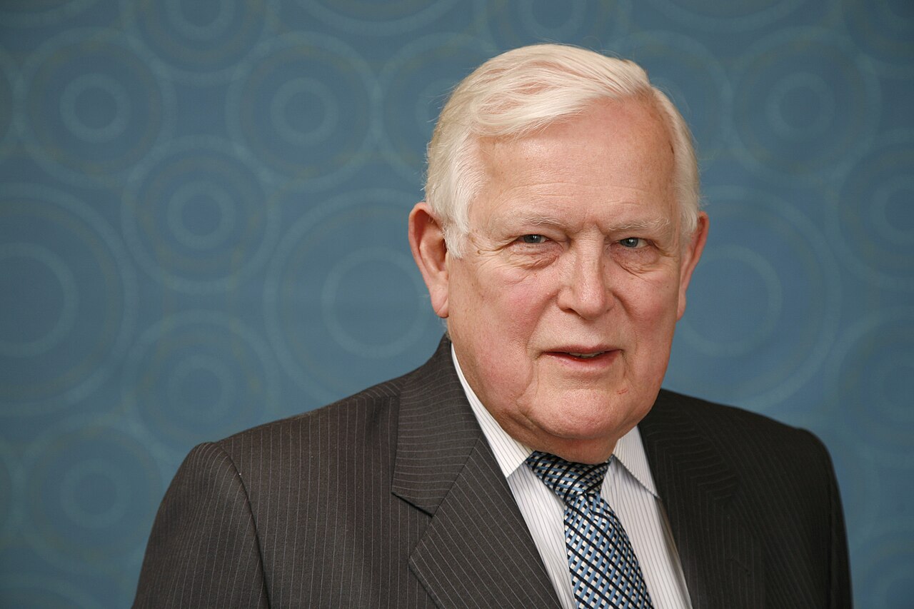
Rudolf Emil Kálmán was born in Budapest on 19 May 1930, the son of Otto and Ursula Kálmán. The family left Hungary in 1943, during the Second World War, and eventually settled in Youngstown, Ohio, where they arrived in 1949. Kálmán spent three years at Youngstown College before he was admitted to MIT to study electrical engineering. He earned his bachelor’s degree there in 1953 and a master’s degree in 1954 under Ernst Guillemin, then moved to Columbia University, where John Ragazzini supervised his doctorate. His 1957 thesis was on “Analysis and synthesis of linear systems operating on randomly sampled data”, the kind of system that digital computers in control loops were creating.
After a short stay at IBM’s research laboratory in Poughkeepsie, Kálmán joined the Research Institute for Advanced Studies (RIAS) in Baltimore in 1958. RIAS was a research center of the Glenn L. Martin Company, and its mathematics division was led by Solomon Lefschetz, who had gathered a group working on differential equations and control. Kálmán stayed until 1964. Nearly all the work for which he is known was done in those six years.
Truth from Noise
Every sensor is inaccurate. A radar return, a gyroscope that drifts, a star sighting by an astronaut: each gives a corrupted view of where a vehicle actually is and how fast it is moving. Estimating that hidden state from a stream of noisy measurements was an old problem. In the 1940s Norbert Wiener and, independently, Andrey Kolmogorov had developed optimal filtering for it. Wiener’s filter worked in the frequency domain, assumed that the signals’ statistics did not change over time, and processed a continuous stream of data. That suited radar fire control. It was hard to apply to a spacecraft whose dynamics change from moment to moment and whose measurements arrive irregularly.
Kálmán worked out his alternative in January 1959. He described the system in state-space form, as a vector of variables (position and velocity, for example) that evolves according to a model and is observed through noisy measurements. His filter is a recursion with two steps. In the prediction step it uses the model to project the current estimate, and the uncertainty of that estimate, forward to the time of the next measurement. In the update step it compares the measurement with what the prediction says it should be and corrects the estimate by a weighted share of the difference. The weight, the Kalman gain, is computed from the two uncertainties: a precise measurement moves the estimate a lot, a noisy one only a little. After each step the filter needs to keep only the current estimate and its uncertainty, not the history of measurements.
The Kalman recursion:

  Predict:  x̂ ← F·x̂                  project the state with the model
            P ← F·P·Fᵀ + Q            and grow its uncertainty
  Update:   K = P·Hᵀ·(H·P·Hᵀ + R)⁻¹   gain from the two uncertainties
            x̂ ← x̂ + K·(z − H·x̂)      correct by part of the surprise
            P ← (I − K·H)·P           and shrink the uncertainty
For linear systems with Gaussian noise this gives the best possible estimate. It needs only a few small matrix operations per measurement, which made it practical on the slow computers of the time.
A Skeptical Reception
Kálmán presented “A New Approach to Linear Filtering and Prediction Problems” at a conference of the American Society of Mechanical Engineers in late March 1959, and it was published in March 1960 in the ASME’s Journal of Basic Engineering. That a paper on signal filtering by an electrical engineer appeared in a mechanical engineering journal reflected the reception it had among the specialists: the state-space approach and its notation were unfamiliar, and the frequency-domain methods of Wiener were established. A second paper, “New Results in Linear Filtering and Prediction Theory”, written with Richard Bucy and covering the continuous-time case, was at first rejected; it was published in 1961.
Kálmán was not the only one to arrive at the idea. Peter Swerling of the RAND Corporation had published a similar recursive method for satellite tracking in 1958. The Danish astronomer and statistician Thorvald Thiele had derived a related procedure for a simpler case in 1880. In the Soviet Union, Ruslan Stratonovich developed a more general nonlinear filter around the same time, of which the Kalman–Bucy filter is a special case, and some authors name it after all three.
In 1960 Kálmán also presented “On the General Theory of Control Systems” at the first congress of the International Federation of Automatic Control in Moscow. It introduced controllability (whether the inputs of a system can steer it to any state) and observability (whether its state can be worked out from its outputs), and showed that the two are mathematically dual. With the filter and his later work on realization theory, these concepts became the basis of what textbooks call modern control theory.
Ames and the Moon
In the autumn of 1959 the Dynamics Analysis Branch at NASA’s Ames Research Center in California, headed by Stanley F. Schmidt, chose to study midcourse navigation and guidance for a circumlunar mission. The branch had eight analysts and an IBM 704. Its plan was for a crew to measure the angles between Earth, Moon and stars with an optical instrument and for an onboard computer to turn those sightings into an estimate of the spacecraft’s position and velocity. The weighted least-squares estimator used by the Jet Propulsion Laboratory was too heavy for any onboard computer of the time and for their own IBM 704. Wiener’s theory, which some of the staff had used for missile guidance, could not handle the nonlinear orbital mechanics or the irregular, discrete measurements.
Schmidt and Kálmán had known each other for several years. In the autumn of 1960 Kálmán, unaware of what the branch was working on, arranged a visit and presented his paper to Schmidt’s staff. The sequential structure was what they needed, since it avoided storing and reprocessing all past measurements. The paper was hard going. Schmidt’s own account says that the notation and the state-space concepts “were also very difficult for practicing engineers to grasp”. On his next trip east, Schmidt met Kálmán at RIAS, and during that meeting he saw how to apply the linear theory to a nonlinear problem: by using the linear perturbation methods his branch already used for guidance.
The Extended Filter
Schmidt’s group had to change Kálmán’s formulation in three ways before it fitted the mission.
- Kálmán’s version assumed measurements at evenly spaced intervals. A crew would take sightings in short bursts separated by long gaps. The Ames team split the filter into a separate time update and measurement update, the predict-and-correct form in which the filter has been taught ever since. Schmidt and McGee later wrote that the decomposition “seems almost trivial” in hindsight but was “a major and critical step forward” at the time.
- They linearized the equations of motion not around a fixed reference trajectory but around the current estimate, recomputing as the estimate improved. A mistake in one simulation run showed how robust this was: the true trajectory stayed in Earth orbit while the filter started out on a lunar transfer, and the estimate still converged to the truth. This version is the extended Kalman filter.
- They wrote all the matrix routines themselves in Fortran, and rewrote them with single indexing because double indexing was too slow on the 704.
When the simulation was ready, one run took a little over an hour on the IBM 704. The first result was disappointing; the cause turned out to be an error in a subroutine call, and the second run worked. By early 1961 the simulations showed that onboard optical measurements could navigate a spacecraft around the Moon with accuracy comparable to least-squares methods, at a fraction of the memory and computation. By luck the team had multiplied the matrices of the update equation in the numerically stable order; the other order produced round-off problems that later teams ran into.
Into Apollo
Early in 1961 Schmidt told Richard Battin of MIT’s Instrumentation Laboratory, which was designing the Apollo guidance system, about the results. Battin had been working along similar lines without knowing Kálmán’s paper. In his report of September 1961 he wrote that “the original application of Kalman’s theory to space navigation was made by Schmidt and his associates.” At MIT, James Potter devised the first square-root formulation of the filter, which kept the computation numerically stable on a computer with short words, and it was used in the Apollo onboard navigation system on the Apollo Guidance Computer.
Schmidt left NASA for Lockheed at the end of 1961. When Lockheed became prime contractor for the C-5A transport aircraft around 1966, the Kalman filter was specified for its navigation system, combining inertial data with radio navigation aids. Schmidt consulted for Northrop on it, and by his account it was the first real-time Kalman filter on board an aircraft. Fighting the round-off problems of fixed-point onboard computers convinced him that a general square-root formulation was needed; he developed one in 1968, and in January 1972 it flew in a NASA landing-navigation system called RAINPAL, the first square-root filter tested in an airborne computer.
Everywhere
From the 1960s the Kalman filter became the standard method wherever a state had to be estimated from noisy sensors:
- Navigation: the navigation systems of the U.S. Navy’s ballistic missile submarines, cruise missiles such as Tomahawk, aircraft inertial systems, and the spacecraft that dock with the International Space Station.
- GPS: receivers combine satellite range measurements with a motion model to produce position and velocity; phones and cars fuse GPS with accelerometers and gyroscopes in the same way.
- Robotics: localization and simultaneous localization and mapping (SLAM) in robots and self-driving cars.
- Weather: ensemble Kalman filters assimilate observations into atmospheric models with millions of variables.
- Economics and signal processing: estimating unobserved quantities such as trends in time series.
The filter’s descendants, among them the unscented Kalman filter and the ensemble Kalman filter, handle nonlinear systems better than the extended version. Particle filters handle the most nonlinear cases by Monte Carlo sampling (see Monte Carlo Methods).
Later Life
Kálmán moved to Stanford in 1964 and in 1971 to the University of Florida in Gainesville, where he directed the Center for Mathematical System Theory. From 1973 he also held the chair of mathematical system theory at ETH Zürich. He retired from both in 1997. He spent much of his later career on system identification, the problem of building models from noisy data, which he considered badly underdeveloped. In his Kyoto Prize address he insisted that “scientific modeling is a deductive exercise, and not a creative act.” In a 1981 lecture on system identification he had already asked of every model whether it was “really based on the data” or an artifact “displaying the prejudices of its creator.”
He received the IEEE Medal of Honor in 1974, the Kyoto Prize in Advanced Technology in 1985, the year the prize was first awarded, the Richard E. Bellman Control Heritage Award in 1997, the Charles Stark Draper Prize in 2008, and the National Medal of Science, presented by President Obama in 2009. He was a member of the U.S. National Academies of Sciences and Engineering and a foreign member of the Hungarian, French and Russian academies. Kálmán died at his home in Gainesville on 2 July 2016, aged 86.
Dead End
The frequency-domain filtering of Wiener and Kolmogorov was the dominant theory of estimation in 1959, and it was the obvious tool for the navigation problem: engineers at Ames had used it for missile guidance for years. For spacecraft navigation it was a dead end. It assumed stationary signals and continuous measurements, it did not handle the nonlinear dynamics of an orbit, and a digital implementation required processing the whole history of the data. The batch least-squares estimators used for ground-based orbit determination worked but needed far more memory and computation than any onboard computer offered. The state-space recursion replaced both for real-time navigation within a few years, and Wiener filtering survived mainly in fields where its assumptions hold, such as the processing of stationary signals in communications and audio.
📚 Sources
- McGee, L. A., and Schmidt, S. F.: “Discovery of the Kalman Filter as a Practical Tool for Aerospace and Industry”, NASA Technical Memorandum 86847 (November 1985): Dynamics Analysis Branch, IBM 704, Kálmán’s visit in autumn 1960, decomposition and extended filter, first runs, Battin quote, Potter’s square-root filter for Apollo, C-5A, 1968 square-root method, RAINPAL flight test January 1972
- Tryphon T. Georgiou, “In Memoriam: Rudolf E. Kalman”, ASME Journal of Dynamic Systems, Measurement, and Control (2017): family, emigration 1943, Youngstown 1949, MIT and Columbia, IBM and RIAS, idea of January 1959, March 1959 presentation, rejection of the Kalman–Bucy paper, IFAC 1960, positions, Kyoto address, the 1981 lecture “System identification from noisy data”, academies, awards, death
- Kalman, R. E.: “A New Approach to Linear Filtering and Prediction Problems”, Journal of Basic Engineering 82(1): 35–45 (1960)
- Wikipedia: Rudolf E. Kálmán and Kyoto Prize: Rudolf Emil Kalman
- Wikipedia: Kalman filter: Thiele, Swerling, Stratonovich, Schmidt’s implementation, submarine and cruise-missile navigation, ISS docking
- Wikipedia: Kyoto Prize: first awarded in 1985
- “Honoring a legacy algorithm”, Aerospace America (AIAA)
- Grewal, M. S., and Andrews, A. P.: “Applications of Kalman Filtering in Aerospace 1960 to the Present”, IEEE Control Systems Magazine 30(3) (2010)
- Image: ETH-BIB-Kalman, Rudolf E. (1930-2016)-HK 04-01925.jpg, CC BY-SA 4.0, via Wikimedia Commons