Monte Carlo Methods

Abstract

In 1946 the mathematician Stanisław Ulam, recovering from a serious illness, wondered what the chances were of winning a game of solitaire. The combinatorics were hopeless, but he realized that he could simply play a hundred games and count. With John von Neumann he turned the idea into the Monte Carlo method: solving problems too complex for exact mathematics by random sampling. Nicholas Metropolis named it after the casino where Ulam’s uncle gambled. In April 1948 a program designed by John and Klára von Neumann ran Monte Carlo simulations of a nuclear weapon core on ENIAC, the first program run in the modern stored-program style. The Metropolis algorithm of 1953 founded Markov chain Monte Carlo, which later made Bayesian statistics practical. Monte Carlo methods now run in reactor design, financial risk models, weather forecasting, film rendering and the search behind AlphaGo. Their weak point was randomness itself: von Neumann’s first generator was flawed, and IBM’s RANDU corrupted a generation of simulations.

Solitaire and the Bomb

Random sampling as a way to compute had precedents: in 1777 the Comte de Buffon showed that dropping needles on a lined floor could estimate π, and Enrico Fermi had used hand-sampled neutron histories in Rome in the 1930s without publishing the method. It became a general tool at Los Alamos after the war.

Stanisław Ulam, a Polish-born mathematician who had worked on the Manhattan Project, was recovering in 1946 from encephalitis when he started to wonder about the probability that a game of Canfield solitaire could be won. Counting the possible deals and moves exactly was hopeless. Playing many games and counting the successes was easy and answered the question well enough. He saw at once that the same approach fitted the problem Los Alamos actually had: neutron diffusion, the way neutrons in a nuclear weapon scatter, are absorbed or cause further fissions, a chain of probabilistic events too tangled to solve analytically.

Ulam described the idea to John von Neumann, who worked out how a computer could carry it out. The machine would follow thousands of individual neutrons one at a time, deciding at each step by drawing a random number whether the neutron collided, was absorbed or caused fission, and the physics would emerge from the statistics. Nicholas Metropolis proposed the name Monte Carlo, after the casino in Monaco where Ulam’s uncle used to go to gamble with money borrowed from relatives. Metropolis and Ulam published the first account of the method, “The Monte Carlo Method”, in the Journal of the American Statistical Association in 1949.

FERMIAC

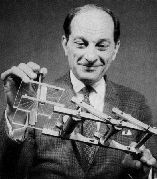
Stanisław Ulam holding the FERMIAC, the hand-pushed analog device Enrico Fermi designed in 1947 to trace neutron paths by the Monte Carlo method. Image: Los Alamos National Laboratory, public domain, via Wikimedia Commons.

While Los Alamos waited for computer time, Fermi built a mechanical substitute. The FERMIAC, constructed by Percy King in 1947, was a small trolley that an operator pushed across a scale drawing of a nuclear device, setting its direction and distance for each neutron step from a table of random numbers and marking the paths on the drawing. It was used for about two years, and it showed the method working before the computers were ready.

ENIAC, April 1948

The first electronic Monte Carlo calculations ran on ENIAC, which had by then been moved from Philadelphia to the Army’s Aberdeen Proving Ground in Maryland. ENIAC had been built to be programmed by setting switches and plugging cables. For the Monte Carlo work it was converted to run programs written as sequences of numeric instructions stored in its function tables, a form much closer to the stored-program design of von Neumann’s EDVAC report.

The historians Thomas Haigh, Mark Priestley and Crispin Rope reconstructed what happened from machine logs and notes. Much of the planning and coding of the Monte Carlo program was done by Klára Dán von Neumann, John von Neumann’s wife, who had learned programming for the project. The von Neumanns came to Aberdeen on 8 April 1948, and Klára stayed for a month to work with Metropolis, who had already reconfigured ENIAC for the new style of programming. The first successful production run came on 17 April; hardware troubles delayed serious work until 28 April, and by 10 May the calculations were finished. It was the first computerized Monte Carlo simulation, and the first program in the modern style ever executed. The calculations of fission weapon cores set the pattern for the hydrogen-bomb work that followed: where the mathematics could not be solved, it was sampled.

The Metropolis Algorithm

In 1953 Metropolis, Arianna Rosenbluth, Marshall Rosenbluth, Augusta Teller and Edward Teller published “Equation of State Calculations by Fast Computing Machines”, which they had run on Los Alamos’s MANIAC computer. Instead of sampling independent random configurations, which would almost never land in the physically likely states of a system of many interacting particles, their method took a random walk: propose a small random change, accept it if it lowers the energy, and accept it with a calculated probability if it raises it. The walk visits states in proportion to their probability in the long run. Arianna Rosenbluth wrote the program for MANIAC (see Women in Computing).

This was Markov chain Monte Carlo (MCMC). Wilfred Hastings generalized it in 1970, and the Gibbs sampler, introduced for image restoration by Stuart and Donald Geman in 1984, gave a simple version for many-variable problems. In 1990 Alan Gelfand and Adrian Smith showed in the Journal of the American Statistical Association that these samplers could compute the posterior distributions of Bayesian statistics, which until then had been intractable for realistic models. Bayesian methods spread through statistics, epidemiology, genetics, physics and ecology in the following decade.

From Neutrons to Everything

The method spread with cheap computing:

Physics and engineering: reactor and shielding design, particle transport in detectors at CERN and elsewhere, semiconductor device simulation.
Finance: option pricing and risk measures such as Value-at-Risk are computed by simulating thousands of possible paths of markets; pension and insurance models work the same way.
Graphics: path tracing, the physically based rendering used in film visual effects and in GPU ray tracing, is Monte Carlo integration over the paths light can take.
Weather and climate: ensemble forecasts run a model many times from slightly different starting conditions, and a “70 percent chance of rain” is the fraction of runs that produced rain.
Games and AI: Monte Carlo tree search, which estimates the value of a move by playing out many random games, made computer Go competitive in the late 2000s and was the search component of AlphaGo. Sampling methods run throughout probabilistic machine learning.

The bargain is the same in every case. An exact answer is often unobtainable; a sampled answer is approximate, but its error shrinks predictably, in proportion to one over the square root of the number of samples, so accuracy can be bought with computing time.

Random Numbers

A sampling method is only as good as its randomness, and producing random numbers on a deterministic machine turned out to be a problem in its own right. Tables were one answer: in 1947 the RAND Corporation built an “electronic roulette wheel” from a pulse generator and used it to produce A Million Random Digits with 100,000 Normal Deviates, published as a book in 1955. Tables, though, were slow to read into a computer and limited in length.

Von Neumann proposed computing the numbers instead, with the middle-square method: square a number, take its middle digits as the next value, and repeat. He knew the weakness. “Any one who considers arithmetical methods of producing random digits is, of course, in a state of sin,” he wrote in 1951. Middle-square sequences fall into short cycles or decay to zero, depending erratically on the starting value. He used it anyway because it was fast and its failures were visible, whereas hardware noise generators could neither be checked nor replayed.

Dead End

The longest-lasting failure was RANDU, a linear congruential generator distributed by IBM for its System/360 computers in the 1960s and copied widely. Each number was the previous one multiplied by 65,539, modulo 2^31, a choice made for speed on binary hardware. It looked random in one or two dimensions. But if consecutive triples of its output were plotted as points in three-dimensional space, all of them fell on just 15 parallel planes. Any simulation that used three or more random numbers together, which included most physical simulations, sampled only a thin set of slices of the space it was meant to explore. Donald Knuth called it “truly horrible”, and the results of many simulations of the 1960s and 1970s that relied on it became suspect.

The episode helped turn random number generation into a field of its own, with statistical tests such as the spectral test that exposed RANDU, and with generators designed against them, from better linear congruential generators to the Mersenne Twister of Makoto Matsumoto and Takuji Nishimura (1997), with a period of 2^19937 − 1, which became the default in many programming languages, and on to the cryptographically secure generators used today.